ABSTRACT
From visual and photoelectric data, a sky brightness - population function for cities and a sky brightness - distance function for average atmospheric conditions are obtained. These functions are used in a simple mathematical model to calculate levels of light pollution over Ontario. From direct observations and model calculations, there are few observing sites free of light pollution in southern Ontario and these will degrade rapidly in the future.
Introduction. The spread of artificial lights in Ontario has become a serious obstacle to professional and amateur astronomers alike. Despite its importance, however, light pollution has been little studied, perhaps because of the reluctance of astronomers (and physical scientists in general) to study man-made phenomena. But light pollution is of such importance today that it cannot be ignored. The study reported in this paper has been undertaken to assess the amount and distribution of artificial light in Ontario skies by seeking the relation of the light emission of cities to their population and the attenuation of this light with distance from the cities. These relationships are then used to calculate light pollution levels over the entire province.
Review of Previous Work. Several useful papers about light pollution have been published, most notably Riegel (1973) and Walker (1970, 1971, 1973). Their work pertains mainly to light pollution around the major observatories in the American southwest. Riegel gives a general introduction to the problem of light pollution and the impact it has on astronomy. Walker's papers are concerned with siting future observatories and with rules of thumb for locating presently unpolluted skies. They also give light-pollution maps of California and Arizona. Bertiau et al. (1973) and Treanor (1973) present a model of light propagation in the atmosphere and a calculated map of light pollution for Italy. Their model forms a partial basis for the work in this paper. Normandin (1974) has obtained data for the siting of an observatory in the province of Quebec. She has derived a brightness - population function and a brightness - distance function that agree well with our results in Ontario.
Light Pollution and Public Awareness. "Light Pollution" means the overall brightening of the night sky by man-made lighting, not the glare caused by luminaries near the observer (such as a neighbour's back porch light), except insofar as these contribute to the illumination of the whole sky. Light pollution is thus a large-scale problem, because a small town can light an area of several hundred square kilometres; and a difficult problem, because officials who have lights installed feel completely justified in doing so (see Public Lighting Needs and IES Lighting Handbook). The problem is complicated by public ignorance: so few people - including amateur astronomers - know what a natural night sky looks like, know what they are losing. Articles in semipopular periodicals (Lovi 1972, Nelson 1973, Weyman 1973, Hoag 1972, Neff 1974, Roosen and Marsden 1975) have spread awareness among professional and amateur astronomers, but the general public remains oblivious to the damage being done. Indeed, in the case of light pollution, as distinguished from other kinds of pollution of the environment, the society at large does not value what is being destroyed (Lopez 1975).
The Sky Brightness Programme. The Sky Brightness Programme of the Toronto Centre of the R.A.S.C. was instituted during the summer of 1974 under the auspices of the Observational Activities Committee to measure and evaluate the extent of light pollution and the quality of the night sky in Ontario. An announcement appeared in the National Newsletter (Dec. 1974) of the R.A.S.C. inviting Canada-wide participation. The methods used for making measurements are briefly described in a later section of this paper. Data for Ontario were collected for about one year, from August 1974 to September 1975. The major features of our model of light emission by cities and its propagation through the atmosphere were developed very quickly, and much of the subsequently accumulated data was used for refining and testing the predictions of preliminary models. The collection of data in the Programme continues; these will be used for the study of seasonal variations, lunar lighting, etc., and for further testing of the model. We intend to develop a more sophisticated model in the future and also to extend the work to cover more of Canada.
TABLE 1 APPEARANCE OF THE SKY AT GIVEN LEVELS OF LIGHT POLLUTION
| Pollution Level in S10 Units | Visual Mag/Arcsec2 (Natural Background=250 S10 Units) | Naked-Eye Appearance of the Sky (M.W. = Milky Way) |
| 0 | 21.7 | The sky is crowded with stars, extending to the horizon in all directions. In the absence of haze the M.W. can be seen to the horizon. Clouds appear as black silhouettes against the sky. Stars look large and close. |
| 20 | 21.6 | Essentially as above, but a glow in the direction of one or more cities is seen on the horizon. Clouds are bright near the city glow. |
| 100 | 21.1 | The M.W. is brilliant overhead but cannot be seen near the horizon. Clouds have a greyish glow at the zenith and appear bright in the direction of one or more prominent city glows. |
| 500 | 20.4 | To a city dweller the M.W. is magnificent, but contrast is markedly reduced, and delicate detail is lost. Limiting magnitude is noticeably reduced. Clouds are bright against the zenith sky. Stars no longer appear large and near. |
| 2000 | 19.5 | M.W. is marginally visible, and only near the zenith. Sky is bright and discoloured near the horizon in the direction of cities. The sky looks dull grey. |
| 5000+ | 18.5 | Stars are weak and washed out, and reduced to a few hundred. The sky is bright and discoloured everywhere. |
Measurement of Sky Brightness. Astronomical surface brightness is commonly expressed among astronomers in terms of stellar brightness per unit area. The unit "magnitudes per square arc-second" is generally used in small-area photometry and in measurements related to stellar physics such as isophotometry of galaxies. The scale is logarithmic, as are all magnitude scales.
The other commonly used unit, "tenth magnitude stars per square degree", usually occurs in large-area photometry such as studies of the Milky Way and zodiacal-light photometry. This unit is linear and relatively easy to visualize. Primarily because of its linearity, it is chosen as the basic unit in this paper. Tables I and II give equivalents which will help those unfamiliar with these units of sky brightness to visualize them.
TABLE II EQUIVALENT MEASURES OF THE SKY BRIGHTNESS
| Equivalent | Magnitude Units | |
| Light Pollution | No Background | 250 S10 Background |
| in S10 Units | mag/arcsec2 | mag/arcsec2 mag/deg2 |
| 0 | -- | 21.7 4.0 |
| 20 | 24.5 | 21.6 3.9 |
| 50 | 23.5 | 21.5 3.8 |
| 100 | 22.8 | 21.4 3.7 |
| 200 | 22.0 | 21.1 3.4 |
| 320 | 21.5 | 20.9 3.2 |
| 500 | 21.0 | 20.6 2.9 |
| 1,000 | 20.2 | 20.0 2.3 |
| 2,000 | 19.5 | 19.4 1.7 |
| 5,000 | 18.5 | 18.5 0.8 |
| 20,000 | 17.0 | 17.0 -0.7 |
| 1 S10 unit | = 1 10th mag star/deg2 |
| = 10.00 mag/deg2 | |
| = 27.78 mag/arcsec2 | |
| = 2.3 x 10⁻⁷ millilambert | |
| = 7.2 x 10⁻¹¹ stilb | |
| = 3.6 x 10⁻³ rayleigh/angstrom at 5500A |
Two photoelectric photometers have been used, one a portable photometer to be used on automobile trips and the other for standardizations. The former photometer consists of an inexpensive 1P21 photomultiplier mounted in a watertight box, fed by a 50 mm simple lens of 100 mm focal length. A metal stop limits the held of view to 9 degree, and a yellow filter gives approximately visual response. The instrument is well baffled to prevent interference from other cars when used on the roof of an automobile. The standardization photometer uses a better quality 1P21 photomultiplier in a watertight housing incorporating a 50 mm focal length Fabry lens. The objective is a 60 mm lens of 400 mm focal length. Standard B and V filters are used. A field of view of 1 degree is normally used because the middle calibration levels of the low-brightness source then give nearly the same deflections as the standard stars used.
The electronics of the photoelectric photometers are run from battery power supplies; the stabilized high-voltage power supply from +/- 18 volts (lantern batteries) and the electrometer amplifier (based on the LH0042 FET input operational amplifier) from +/- 9 volts (transistor batteries).
The low-brightness source is a wooden box 20 cm square and 60 cm long. A lamp in the rear illuminates a small opal glass screen. Ten apertures from 1 mm to 30 mm placed in front of the screen allow control of the light shining on a 17 cm square of opal glass at the front of the box. A brightness range of 1:1000, or 7 1/2 magnitudes, is attained.
Standardization. To standardize the low-brightness source, two stars of around first magnitude were observed on several nights in both V and B over four- to six-hour periods as they rose in the sky, these observations being interspersed with observations of the low-brightness source. The average stellar extinction coefficients determined kv = 0.22, kB = 0.36 were used to correct for atmospheric extinction the deflections produced by the stars. Knowing the field of view of the photometer and the catalogue brightness of the stars, we then calculated the surface brightness of the low-brightness source. The readings of the standardization photometer, when observing the low-brightness source, were used as a separate check on the stability of the latter. These remained within 0.05 mag over a six-month period.
Calibration. Calibration of a visual photometer is performed by having the observer measure the entire set of ten low-brightness source values, usually once in descending order of brightness, then twice in random order. A calibration curve consisting of a graph of wedge position reading versus source brightness in mag/sec2 is then constructed. The probable error for a set of three observations is about 0.1 mag at 16 mag/sec2 and grows to 0.3 mag at 22 mag/sec2 for an average observer.
Before and after an observing trip by automobile, the sensitivity of the portable photometer is calibrated against the low-brightness source. This also constitutes a further check on the stability of the low-brightness source. Readings remained within 0.10 mag of expected values during several checks over a six-month period. Considering the rough treatment encountered by the portable photometer, this stability is quite surprising.
Observations.
Dependence of Sky Brightness on Zenith Angle. The zenith-to-horizon variations in intensity of a light-polluted and a natural sky are quite different. The natural sky shows an increase of about 0.5 mag from the zenith to 85 degree zenith angle, this increase being due primarily to the airglow component of the natural sky light (Roach and Gordon 1973). Light-polluted skies, on the other hand, show a very marked increase of 2 mag from the zenith to 80 degree zenith angle, such that the brightness of the sky increases proportionally with the secant of the zenith angle (but only for zenith angles less than 80 degree). The secant law becomes distorted very close to large cities, but it should be noted that the horizon is brighter in directions both toward and away from a city. See Figure l.
Horizon to zenith to horizon (HZH) scans were taken at heavily polluted and natural sites in Ontario and the results are shown in figure 2. Data resulting in curves of similar shape are reported by Walker (1970, 1971, 1973) for observations at light-polluted Mount Hamilton (Lick Observatory) and various dark sky sites in California and Mexico. It should be noted that once the natural sky light becomes insignificant, the shape of the HZH curve remains constant. If city light is uniformly scattered by one or more uniform layers of scattering material, in a transparent medium, the observed brightness of the layer should be proportional to its line-of-sight thickness, which increases as the secant of the zenith angle. The observed departure from a secant law near cities is due partially to forward scattering and partially to the greater intensity of the incident light in the cityward direction. The relatively great brightening at large zenith angles in light-polluted skies is a phenomenon that can serve as a useful diagnostic tool in assessing whether or not there is light pollution at a given site. Figure 3, a photograph taken at Cyprus Lake Park on the Bruce Peninsula, shows only slight brightening at the horizon, indicative of a low level of light pollution.
Population Function. To determine the light output from cities of different populations, we measured the back scattered light from the centres of cities and towns (see figure 4). In small towns (under 5,000) the observations were usually made from an unlighted lot or parking area within 250 m of the main traffic intersection. In larger cities the observations were made from unlighted residential streets near the centre of the city. Because the sky brightness is very greatly increased if the scattering layer is unusually close or opaque (i.e. if fog, haze, or cloud is present) observations are shown for very clear nights only. We find that the downtown zenith brightness of a city is proportional to the square root of its population. A similar conclusion is reached by Normandin (1974) for the zenith sky 8 km outside Quebec towns. Other workers (Walker 1970, 1973; Treanor 1973) have based their work on the assumption that the output is proportional to population, but present no corroborating data. We suspect that in large cities the back scattered light is not proportional to the total output of light by the city since light from distant parts of the city is somewhat attenuated and thus does not contribute fully to the downtown sky brightness. Our data show that small cities, for which the entire city contributes light equally, fit the square root relation reasonably well.
If we assume that light output is directly proportional to population, fitting the observed light levels seen over cities in the 1,000 to 60,000 range, we predict a zenith brightness in downtown Toronto that is a factor of 20 to 100 times higher than observed, depending on the assumptions we make regarding the transfer of light from the more distant parts of the city. Since any light pollution model depends critically upon the assumed relationship with population, a subject of some debate, further study is necessary. The ideal way to determine total light output by cities is by photometry from airplane or satellite altitudes and compilation of complete data on the lighting of cities from the records of their Public Works Departments.
Radial-Distance Function. The decrease in zenith illumination at increasing distances from cities is difficult to measure because the decrease is so rapid that the natural background from other cities and towns soon dominates. Small cities such as Guelph are not bright enough to permit accurate assessment of their contributions to zenith light at distances greater than 20 or 30 km, while large cities such as Toronto are surrounded by interfering suburbs and satellite cities. Observations of the radial-distance function were obtained around Hamilton, Ontario, because it is large enough to be a bright source of light, but has relatively few suburbs. Figure 5 has been constructed from data taken on automobile trips to the south-west along Hwy. 6, to the west along Hwy. 5, and to the north along Hwy. 6. Small towns and the natural background rapidly obscure the contribution of a large city. These data, as well as visual and photoelectric measurements taken at many sites in southern Ontario, were used to define the radial-distance function.
The Mathematical Model. The Sky Brightness Programme model is based on Treanor's (1973) "light propagation law", modified to fit observations obtained in Ontario.
Consider an observer located at O (see figure 6). A layer (or multiple layers) of air above him at Z is illuminated by towns T, only one of which is shown in the figure. The illumination of Z will be taken as proportional to the flux passing through it. From the observational material it is seen that the contribution of a single town to the brightness, B, of the sky at distance D from the town, is:
Although we have empirical data for the function Q, let us consider the functional form we can expect Q to assume. Three effects will presumably operate. First, direct light from the town will decrease in accord with the inverse-square law; secondly, singly-scattered light from points P along the path will reach Z; and third, light will be absorbed in the atmosphere.
The intensity Id of the direct light may be written
The singly-scattered ray is assumed to be scattered uniformly inside a cone of semi-angle ![]() thus all scattered light reaching Z must originate within the figure of revolution generated by arc T Z. This volume is built up from many thin disks with area Sd and of thickness dx at distance x from T, each contributing illumination dIs:
thus all scattered light reaching Z must originate within the figure of revolution generated by arc T Z. This volume is built up from many thin disks with area Sd and of thickness dx at distance x from T, each contributing illumination dIs:
By judicious fitting of the individual terms of (9) to the observational data, we chose the following values for the constants:
Assumptions Implied by the Model. A mathematical model is significant only insofar as it describes a realistic physical situation. Examination of the model shows that it assumes or implies the following picture of reality:
Determination of the Constants Used in the Model. The constants a, U, V, h and k were determined by fitting the model to suitable Sky Brightness Programme data. Upon examination of equation (9) , it is seen that all five constants need not be fitted simultaneously, since under certain conditions the equation may be simplified:
The final values of k and h are in reasonable agreement with values in the literature and represent reasonable values for the average optical properties in the tropospheric aerosol mixing layer (Rozenberg 1966, Elterman 1966, 1970, Eppers 1968, Divari 1970).
The values of U and V are markedly different from the values used by Treanor (1973) in that Treanor finds a very much higher level of scattered light. However, he has assumed a different population function, in effect decreasing the importance of satellite cities and giving the appearance of additional scattered light. In principle, the ratio of direct to scattered light could be measured directly from an airplane, but this would pose substantial experimental difficulties.
Production of a Light-Pollution Map. The greatest value of the model is its predictive power, i.e. the ability to calculate light pollution at specified sites with the aim of the selection of possible good ones. To this end we have produced light pollution maps in both coded grey scale and isophote forms. The mathematical model was applied to Ontario, including contributions from nearly all cities over 1,000 population in Ontario and large cities in adjacent areas of Quebec, New York, Michigan, Ohio, and Pennsylvania. Some 325 cities and towns were considered. Ontario was divided into 6,000 blocks, each 8 km square, and the light contributed by all of the cities was calculated for each block using a PDP-45 computer. A detailed description of the method is found in Pike (1976).
Figure 8 and figure 9 are contour maps produced from a numerical listing of light-pollution levels in each 8 km block. Five sky brightness isophotes are shown (20, 100, 200, 500 and 1,000), enclosing the five critical levels of sky quality defined in Table I. Extra contours (50 and 320) are shown in areas where the local structure of light pollution may play a role in site selection. The isophotes refer to the visual region of the spectrum and average meteorological conditions. Note that the natural background level is around 250 to 300 S10 units at deep-sky sites in Ontario with no moon and in the absence of auroral activity. (Refer to Table II for conversion of these light-pollution levels to the conventional units of magnitudes per arcsec2). The values of the contour levels should be increased approximately 10% per year after 1975 to compensate for the increase of population and light.
Seriousness of Light Pollution. Light pollution affects all populated parts of Ontario; few people, thus few astronomers, live in regions where the sky can be considered non-degraded. Light pollution is so prevalent, in fact, that many amateurs of high school age have never seen a non-degraded sky and react to rather badly degraded skies with great excitement. The loss of the natural sky is largely unnoticed by those not acquainted with astronomy.
The cost of commercial and outdoor lighting in terms of energy is great, since lighting accounts for around 20% of total electric power consumption (MacAdam 1975) and night outdoor lighting takes a large fraction of this. Riegel (1973) states that outdoor lighting levels in the U.S. are growing at about 20% per year, many times faster than the population. Riegel gives five reasons for the rapid growth rate:
We have attempted to assess the growth rate of light pollution and find that an annual increase of about 10% is consistent with available data. It is worth noting that in 1935 the Milky Way could be seen in downtown Toronto (Hogg 1975)! Pike (1976) has made extrapolations of light pollution levels in Ontario for the next 25 years. Unless the trend changes drastically, it is evident that few reasonably accessible dark-sky sites will remain by the end of the century, and that suburban and semi-rural skies will be seriously damaged by light pollution.
The most effective limit to the growth of light levels may he the need for energy conservation and more efficient use of light sources (MacAdam 1975), including the use of shields and reflectors to direct less light upward (Hoag and Peterson 1974).
Conclusions.
We have obtained data from visual and photoelectric instruments to define a population-brightness function for cities and a distance-brightness function for average atmospheric conditions in Ontario. We have used these functions to construct a simple mathematical model of light pollution in Ontario. Data from many locations indicate the model gives essentially correct results. We find, from direct observation and model calculations, that there are very few observing sites in southern Ontario unaffected by light pollution, and that these will degrade rapidly in the future. We fear that, within a few decades, there will be virtually no opportunity for anyone to view the natural sky in southern Ontario, which will be a great loss to our culture, as well as to astronomy and star-gazing.
Acknowledgments. I would like to thank all the observers who contributed to this project, in particular, Robert Burnham, Andreas Gada, Keith Hadley, Steven Morris, and Robert Pike for their continued and systematic observations. Extra thanks go to Robert Burnham and Steven Morris for their aid in compiling the bibliography, and to Robert Pike for his computer programming skills. The Toronto Centre of the R.A.S.C. has provided funds through the Observational Activities Committee for the publications issued by the Sky Brightness Programme.
REFERENCES
| Berry, R.L. | 1974, A Manual for the Study of Light Pollution in the Night Sky, Toronto Centre,R.A.S.C. |
| Berry, R.L. and Pike, R.C. | 1975, Observer's Booklet, Toronto Centre, R.A.SC. |
| Bertiau, F.C., S.J., de Graeve, E., S.J and Treanor, P.J., S.J. | 1973, Vatican Obs. Publ., 1, No. 4. |
| Divari, N.R. | 1970, ed., Atmospheric Optics (Consultants Bureau, Plenum Publ.. New York). |
| Ellerman, L. | 1966, Appl. Optics, 5, 1769. |
| Elterman, L. | 1970, ibid., 9, 1804. |
| Eppers, W. | 1968, in C.R.C. Handbook of Lasers (Chemical Rubber Co., Cleveland), p. 39. |
| Hoag, A.A. | 1972, Mercury, 1, No. 5, 2. |
| Hoag, A,A, and Peterson, A.R. | 1974, Observatories and Outdoor Lighting, AURA Report, Kitt Peak National Observatory. |
| Hogg, H.S. | 1975, private communication. |
| ed. J. Kaufman | 1972; IES Lighting Handbook, (Fifth Ed.). (Illum. Eng. Soc., New York). |
| Lopez, B. | 1975, Audubon, July, p. 18. |
| Lovi, G. | 1972, Sky and Telescope, 44, 98. |
| MacAdam, D.L. | 1975, J.O.S.A., 65, 1088 |
| Neff, J.S. | 1974, Mercury, 3, No. 1, 8. |
| Nelson, R. | 1973, ibid., 2, No. 1, 2. |
| Normandin, M. | 1974, Appendix D in Demande d'Octroi au Conseil National de Recherches du Canada pour l'Installation d'un Observatoire Astronomique au Qu�bec, Universit� de Montr�al,Montr�al. |
| Pike, R. | 1976, J.R.A.S. Canada, 70, 116. |
| Pritchard, B.S. and Elliott. W.C. | 1960, J.O.S.A.. 50, 191. |
| Public Lighting Needs 1966 | by Joint Committee of the Institute of Traffic Engineers and Illumination Engineering Society, Illum. Eng., 61, 585. |
| Riegel, K.W. | 1973, Science, 179, 1285. |
| Roach, F.E. and Gordon, J.L. | 1973, The Light of the Night Sky (D. Reidel, Dordrecht and Boston). |
| Roosen, R.G. and Marsden, B.G. | 1975, Sky and Telescope, 49, 363. |
| Treanor, P.J., S.J. | 1973, Observatory, 93, 117. |
| Weyman, R. | 1973, Mercury, 2, No. 2, 2. |
| Walker, M.F. | 1970, Pub. A.S.P., 82, 672. |
| Walker, M.F. | 1971, ibid., 83, 401. |
| Walker, M.F. | 1973, ibid., 85, 508. |
Return to RASC home page
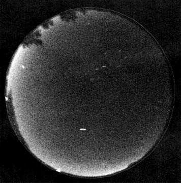
Figure 1 - Fish-eye photograph of the night sky at Palermo, Ontario. Note the brightening at the horizon.
Figure 2 - Horizon-zenith-horizon scans, on the meridian, of five
night skies: a) downtown Toronto, March 20, 1975; b) Palermo, Ontario,
September 16, 1974; c) Lynden, Ontario, September 14, 1974; d) Cyprus
Lake Provincial Park, September 6, 1975; e) Junipero-Serra Peak,
California, from Walker (1973).
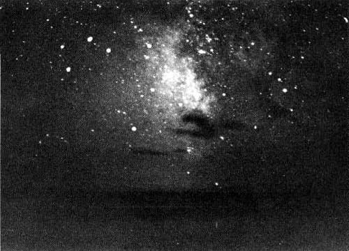
Figure 3 - Appearance of a non-polluted sky near the horizon. The
photograph was taken at Cyprus Lake Provincial Park on the Bruce
Peninsula.
Figure 4 - The relation between downtown sky brightness at the
zenith and population for twelve Ontario cities and towns. The straight
line is the square-root proportionality described in the text.
Figure 5 - Schematic model used in deriving the Q function. See the text for an explanation of the terminology.
Figure 6 - Schematic model used in deriving the Q function. See the text for an explanation of the terminology.
Figure 7 - The attenuation function, Q (heaviest line), the dissection (U/X2) and scattered (V/X) components (light lines), and their sum.
Figure 8 - Contour map of light pollution in south-western Ontario. Solid areas represent urban use. Contour levels are in S10 units.
Figure 9 - Contour map of light pollution in south-western Ontario. Solid areas represent urban use. Contour levels are in S10 units.
Return to RASC home page